What caught my attention
What caught my attention
I started looking at Anthropic because of the discussion around its IPO.
The obvious question is valuation.
How much is a company like Anthropic worth when revenue is growing this quickly?
But that was not the part that stayed with me.
What caught my attention was the other side of the story.
Anthropic is not only building models and selling access to Claude.
It is also securing enormous amounts of physical compute.
In April 2026, Anthropic said it had committed more than $100 billion over ten years to AWS, securing up to 5 GW of capacity. It has also announced a $30 billion Azure compute commitment, alongside large agreements with other infrastructure providers.
There is a good reason for this.
Compute is a constraint.
If customer demand grows faster than available capacity, Anthropic cannot simply wait for new infrastructure to appear.
Capacity has to be planned.
Data centres have to be built.
Chips have to be secured.
Power has to be available.
Many of these decisions have to be made before the future demand is known.
And this is where I became interested.
The physical commitment can extend for years.
But our visibility into the technology may be much shorter.
Model leadership can change.
Inference costs can fall.
Customers can switch.
New chips can arrive.
The amount of compute required for the same task can change.
Even the way we use AI may look different two years from now.
So I started with a simple question:
What happens when the duration of a compute commitment becomes much longer than the duration of our confidence in the economics behind it?
My first intuition was to call this a duration mismatch.
And then another question followed.
If that mismatch becomes large enough, does the downside remain proportional?
Or can a relatively small change in demand eventually create a much larger financial effect?
That is the question I want to explore in this note.
The commitments are long. But how long is the risk?
At first sight, the numbers look simple.
Anthropic has committed more than $100 billion over ten years to AWS.
The agreement secures up to 5 GW of compute capacity.
Anthropic has also committed to purchase $30 billion of Azure compute capacity.
These are large numbers.
They also extend far into the future.
My first reaction was therefore simple.
Anthropic appears to be making long-duration commitments against a technological environment that can change much faster.
But there is a problem with this interpretation.
A ten-year agreement does not necessarily create ten years of economic risk.
The important question is not only how long the contract exists.
It is how long Anthropic is actually locked into it.
Consider the agreement with SpaceX.
SpaceX disclosed that Anthropic agreed to pay $1.25 billion per month for access to compute capacity through May 2029.
That sounds like a very long commitment.
But the same disclosure contains another important detail.
The agreements can be terminated by either party with 90 days’ notice.
That changes the economics completely.
The stated contract horizon extends to 2029.
The effective lock-in can be much shorter.
This distinction matters.
Imagine two compute contracts.
Both have a headline value of $30 billion.
The first cannot be cancelled for five years.
The second can be terminated after six months.
The headline commitment is the same.
The risk is not.
I therefore think we need to separate two ideas.
The first is contractual duration.
This tells us how long the agreement is expected to run.
The second is economic lock-in.
This tells us how long the company remains exposed before it can change the decision.
That exposure depends on more than time.
Cancellation rights matter.
Minimum-spend requirements matter.
Renegotiation rights matter.
The ability to move workloads elsewhere matters.
Even the ability to reuse the compute for another model matters.
In other words, the real risk is not:
It is closer to:
This is a much more useful quantity.
It also prevents us from doing something misleading.
We should not simply add every announced compute agreement together and call the result Anthropic’s fixed liability.
We do not know that.
For some contracts, the relevant terms are not public.
For others, we know that significant optionality exists.
This means that a large headline commitment can still contain flexibility.
And flexibility has economic value.
A company that can exit, resize or redirect capacity after new information arrives is in a very different position from a company that cannot.
This is where the idea of optionality enters the analysis.
The capacity may be committed today.
But the risk depends on how much freedom remains tomorrow.
So before asking whether Anthropic has taken too much duration risk, I think we need a better question:
How much of the announced compute capacity is truly irreversible, and for how long?
Without that distinction, the size of the contracts tells us surprisingly little about the size of the risk.
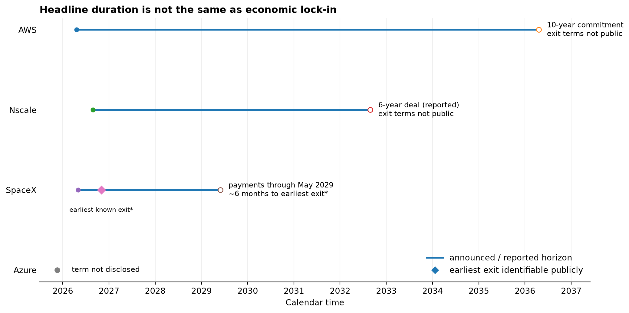
Sources: Anthropic (Anthropic 2026, 2025), SpaceX (Space Exploration Technologies Corp. 2026), and Reuters (Reuters 2026).
The horizontal line shows the publicly announced or reported horizon. It should not be interpreted as the period over which all payments are unavoidable. The diamond for SpaceX shows an approximate earliest exit based on the disclosed initial three-month period followed by 90 days’ notice. For AWS and Nscale, equivalent exit provisions are not public. Azure’s $30 billion commitment has no publicly disclosed term in the announcement.
A demand shock does not stop at revenue
Now suppose some of the capacity is genuinely locked.
What happens if demand turns out to be lower than expected?
The first effect is obvious.
Revenue is lower.
But the financial effect does not necessarily stop there.
Some costs move with demand.
Others do not.
If Anthropic serves fewer requests, some variable compute costs may fall.
But a committed capacity payment may remain.
This creates operating leverage.
A simple model is enough to see it.
Let revenue be
where $ is demand and is the revenue generated per unit of demand.
Now separate the cost base into two parts.
Here, represents costs that move with demand.
represents costs that remain committed over the horizon we are studying.
Operating contribution is then
The important part is .
If demand falls, changes.
But does not.
That creates an asymmetry.
Consider a simple example.
Assume expected revenue is 100.
Variable costs are 30.
Locked capacity costs are 40.
Operating contribution is therefore 30.
Now reduce revenue by 10%.
Revenue becomes 90.
Variable costs fall to 27.
The locked capacity cost remains 40.
Operating contribution becomes 23.
Revenue fell by 10%.
Operating contribution fell by about 23%.
Now reduce revenue by 20%.
Revenue becomes 80.
Variable costs become 24.
Locked capacity remains 40.
Operating contribution falls to 16.
Revenue is down 20%.
Operating contribution is down almost 47%.
Nothing unusual has happened mathematically.
This is simply operating leverage.
The company committed part of its cost base before the demand was known.
When demand is strong, that can work in its favour.
Additional revenue can move quickly into profit.
When demand disappoints, the same structure works in the opposite direction.
This also shows why utilisation matters.
Suppose Anthropic reserves capacity .
Actual demand is .
We can define utilisation as
When is close to one, most of the reserved capacity is being used.
When falls, part of the committed capacity is economically idle.
The cost may still exist.
The revenue does not.
This is the first amplification mechanism in the system.
But I would stop here before calling it convexity.
A fixed cost can make profit move much faster than revenue.
That does not automatically make the relationship mathematically convex.
We need one more mechanism for that.
And that is where the valuation side becomes important.
| Revenue shock | Revenue | Variable cost | Locked cost | Operating contribution | Contribution change | |
|---|---|---|---|---|---|---|
| 0 | 0% | 100.0 | 30.0 | 40 | 30.0 | 0.0% |
| 1 | -10% | 90.0 | 27.0 | 40 | 23.0 | -23.3% |
| 2 | -20% | 80.0 | 24.0 | 40 | 16.0 | -46.7% |
| 3 | -30% | 70.0 | 21.0 | 40 | 9.0 | -70.0% |
The numbers are illustrative. The point is not their magnitude. The point is that a partly fixed cost structure can transform a moderate demand shock into a much larger change in operating contribution.
Fixed costs are not convexity
At this point, it is tempting to call the previous result convex.
I do not think that is correct.
The fixed capacity cost clearly amplifies the effect of a demand shock.
But amplification alone is not convexity.
In our simple model,
operating contribution is still a linear function of demand.
If , , and remain constant, then
and
The second derivative is zero.
So there is no curvature.
There is operating leverage.
But there is no mathematical convexity yet.
This distinction matters.
A company can have very high operating leverage without having a convex payoff.
The percentage change in profit can still be much larger than the percentage change in revenue.
That happens because profit is measured after the fixed cost has already been paid.
But the underlying relationship remains linear.
To create convex downside, something else has to change as the shock becomes larger.
For example, the realized price may fall.
The valuation multiple may compress.
Financing costs may increase.
Customers may leave faster once product quality deteriorates.
A capacity provider may become less willing to renegotiate.
Or a refinancing constraint may suddenly become binding.
These effects are different.
They introduce state dependence.
The response of the system now depends on where the system already is.
A small demand shock may be manageable.
A larger shock may move the company into a different regime.
That is where nonlinear behaviour can begin.
I therefore want to separate two mechanisms.
The first is operating leverage.
The second is nonlinear repricing.
The first mechanism amplifies.
The second can bend the response itself.
That is the point where the word convexity becomes more useful.
So the next question is not whether fixed compute commitments create convexity.
They do not, by themselves.
The better question is:
What additional mechanisms can turn operating leverage into convex downside?
Where the convexity enters
The operating model gives us amplification.
But equity investors do not value the company only on today’s operating contribution.
They value expected future cash flows.
That means a demand shock can affect more than current revenue.
It can also change what investors believe about the future.
Suppose equity value is written very simply as
where is revenue and is the valuation multiple.
This is deliberately simple.
The multiple itself depends on several things.
Growth matters.
Margins matter.
Risk matters.
So we can think of it as
where is expected growth, is expected margin, and represents the required return or perceived risk.
Now consider a demand shock.
Revenue falls.
That part is direct.
But lower demand can also reduce capacity utilisation.
Lower utilisation can compress margins.
A weaker demand trajectory can reduce expected growth.
And once both growth and margins are revised down, the market may also reduce the multiple it is willing to pay.
The same shock is now moving several variables at once.
can lead to
and eventually
This is different from the fixed-cost example.
The response is no longer determined only by the original demand shock.
The state of the company changes as the shock becomes larger.
That change can affect the price investors assign to every remaining dollar of revenue.
Consider another simple illustration.
Start again with revenue of 100.
Assume the company is valued at 15 times revenue.
Its normalized equity value is therefore
Now suppose revenue is 10% below expectation.
If the multiple remains at 15, equity value falls by the same 10%.
There is no additional amplification from valuation.
Now assume the weaker demand also changes the market’s view of growth and margins.
The multiple falls from 15 to 12.
Then
Revenue is down 10%.
Equity value is down 28%.
Now consider a larger demand shock.
Suppose revenue falls 20%.
Margins deteriorate further.
Growth expectations are revised down again.
The multiple falls to 9.
Then
Revenue is down 20%.
Equity value is down 52%.
The initial shock has not doubled.
The equity loss almost has.
This is much closer to what I mean by convex downside.
It is not caused by the valuation multiple alone.
It is created by interaction.
The demand shock affects utilisation.
Utilisation affects margins.
Margins and demand affect expected growth.
Those expectations affect the multiple.
The mechanisms reinforce each other.
This also means that the result is state dependent.
A 10% demand miss when capacity is fully flexible may not matter much.
The same 10% miss with large locked capacity may matter more.
And the same shock can matter even more if the market was already pricing very high growth.
So the relevant question is not simply:
How much does demand fall?
It is:
What else starts moving when demand falls?
That is where the shape of the downside changes.
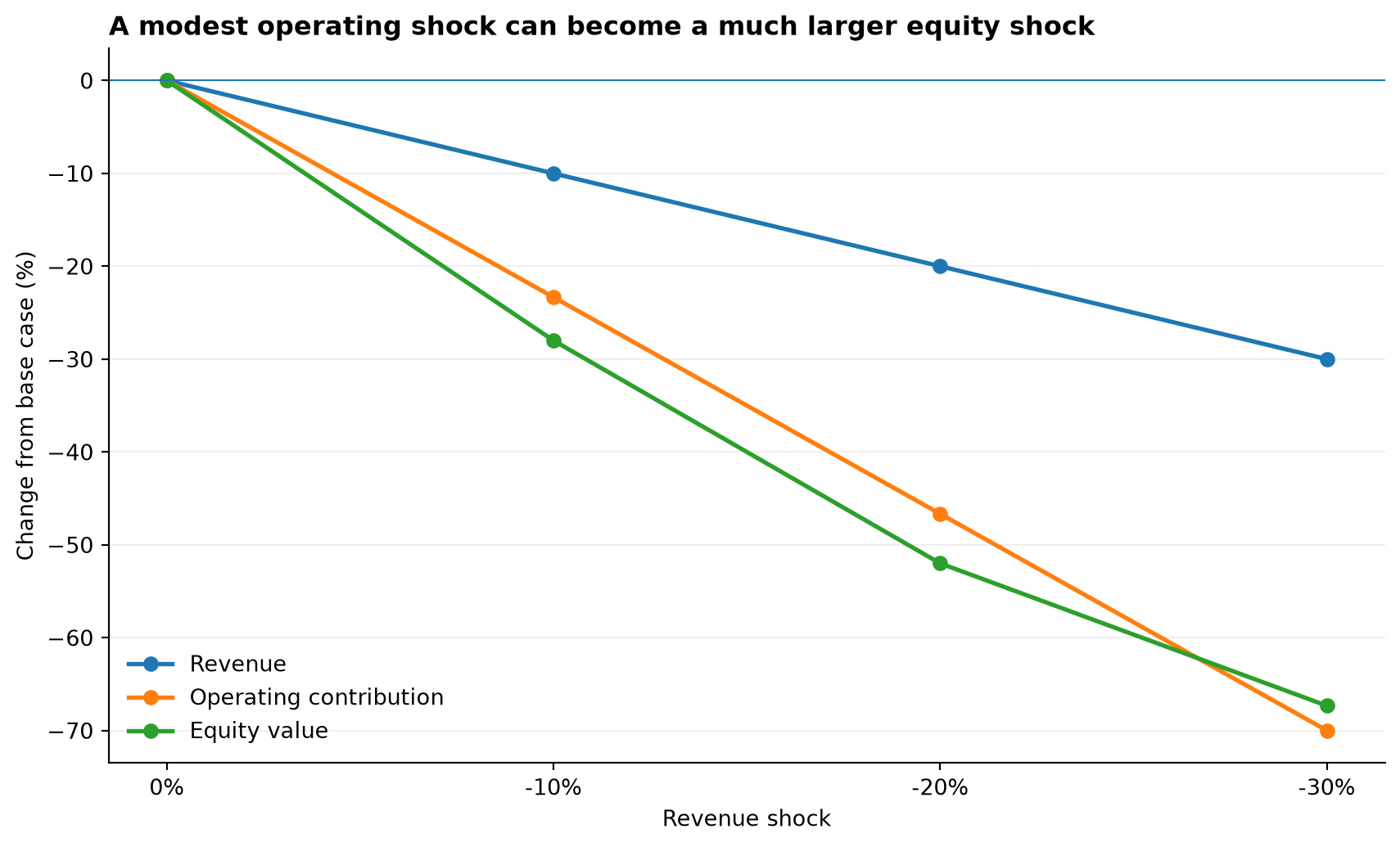
Illustrative stress test. The valuation multiples are assumptions, not estimates for Anthropic. The purpose is to show the mechanism: fixed capacity can amplify the operating shock, while changing expectations can amplify the equity effect again.
Risk does not disappear. It changes hands.
So far, I have treated the compute commitment as an Anthropic problem.
But that is only one side of the contract.
Every payment by Anthropic is revenue for somebody else.
That matters.
Suppose Anthropic commits to a data centre for several years.
The provider now has something valuable.
It has contracted future revenue.
That revenue can support an investment decision.
A data centre can be built.
GPUs can be purchased.
Power can be secured.
Debt can be raised.
The original demand expectation has now travelled further into the system.
This is where I think the problem becomes more interesting.
A contract can transfer risk.
It does not necessarily eliminate it.
Consider a simple chain.
Each layer sees something slightly different.
Anthropic sees customer demand.
The compute provider sees contracted capacity demand.
The infrastructure owner sees expected utilisation.
The lender sees expected cash flow.
These are connected.
But they are not the same thing.
Suppose customer demand turns out to be weaker than expected.
If Anthropic can cancel the capacity, some of the risk moves back to the provider.
The provider may now have unused infrastructure.
If Anthropic cannot cancel, the provider may remain protected.
But Anthropic carries more of the loss.
The contract decides where the first loss sits.
Now add financing.
Assume the provider built the infrastructure partly with debt.
The lender may have assessed the project based on contracted revenue.
As long as the contract performs, this can look stable.
But if the contract is renegotiated, cancelled or impaired, the lender is no longer exposed only to a data centre.
The lender is indirectly exposed to the economic assumptions behind AI demand.
This creates a form of hidden concentration.
Different loans can finance different data centres.
Different funds can hold different securities.
Different providers can appear to have different customers.
But the underlying economic exposure may still depend on a relatively small number of AI companies.
S&P Global has pointed to this issue in AI infrastructure finance.
The financing is increasingly spread across private credit, asset-backed finance, CMBS, ABS and corporate debt.
The instruments look different.
The underlying demand can still be concentrated.
That is an important distinction.
Diversification of securities is not necessarily diversification of economic risk.
I would therefore describe the propagation in four stages.
First, there is a demand shock.
Customers use less AI than expected, or they pay less for it.
Second, there is a utilisation shock.
Reserved or constructed compute capacity is used less intensively.
Third, there is a cash-flow shock.
Someone in the chain earns less than originally expected.
Finally, there can be a financing shock.
Debt service becomes harder.
Refinancing becomes more expensive.
Collateral values may fall.
New projects become harder to finance.
The important point is that these stages are conditional.
A demand shock does not automatically become a credit event.
There are buffers in between.
Contracts are one buffer.
Cash reserves are another.
Equity capital absorbs losses.
Diversified customers help.
Low leverage helps.
Flexible capacity helps.
But the more rigid the contracts become, and the more leveraged the infrastructure becomes, the further the shock can travel.
This suggests another simple way of looking at the system.
The important variable is not only the amount of compute being built.
It is also who has promised what to whom, for how long, and with how much leverage behind that promise.
That is where risk can accumulate quietly.
And it leads to the next question.
If the same demand assumptions are embedded across many contracts, projects and lenders, when does a company-level problem start to look like a system-level problem?
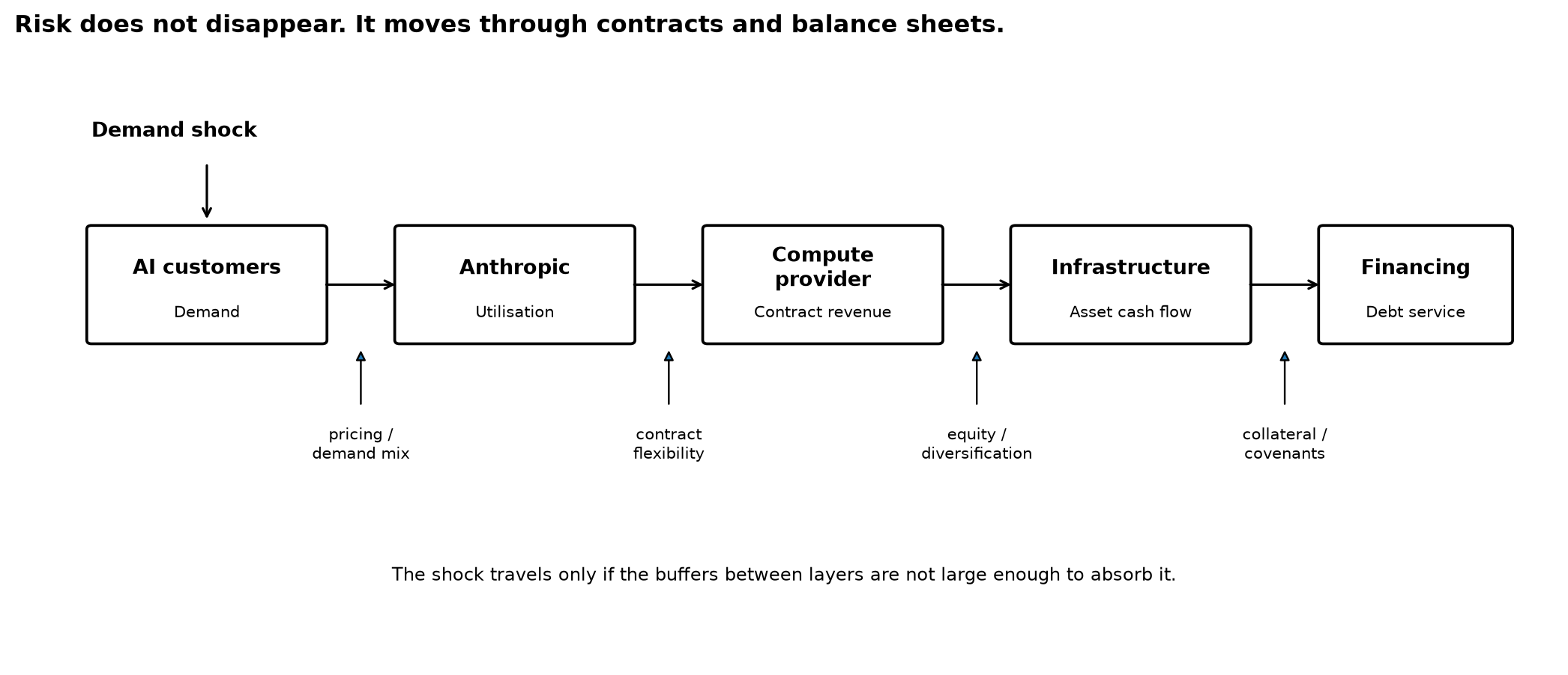
This is a causal map, not an estimate of loss probabilities. The arrows show possible transmission channels. They do not imply that a shock at Anthropic would necessarily reach lenders.
Is this a 2008 problem?
Once risk starts moving through contracts and balance sheets, the comparison with 2008 becomes tempting.
I think we should be careful with it.
A large corporate loss is not a financial crisis.
A failed data centre is not a financial crisis either.
Even several failed AI infrastructure projects would not automatically make the problem systemic.
Something else is required.
The 2008 crisis was not caused only by falling house prices.
The financial system had built a structure around those prices.
Leverage was high.
Short-term funding was fragile.
Many institutions held similar exposures.
Balance sheets were interconnected.
When losses appeared, institutions tried to reduce risk at the same time.
That created forced selling.
Forced selling reduced asset prices.
Lower prices weakened balance sheets further.
The initial shock became a feedback loop. The Federal Reserve later identified leverage, maturity transformation, correlated exposures and interconnectedness as central vulnerabilities that allowed relatively localized losses to propagate through the financial system.
That distinction is useful here.
The trigger and the vulnerability are not the same thing.
For AI infrastructure, a trigger could be simple.
AI demand grows more slowly than expected.
Pricing falls faster than expected.
A new model requires less compute.
A major customer changes provider.
A large capacity contract is renegotiated.
None of these events is necessarily systemic.
The more important question is what structure has been built around them.
Suppose a data centre is financed mostly with equity.
Demand falls.
The owners lose money.
The asset may be worth less.
But the loss can stop there.
Now suppose the same asset has substantial debt.
Its valuation depends on high utilization.
Its debt needs refinancing.
Its lender has similar exposures elsewhere.
And several projects depend on the same small group of AI customers.
The same demand shock now has a different meaning.
This is why leverage matters.
It determines how much loss the equity buffer can absorb before somebody else is affected.
Funding structure matters too.
Long-lived infrastructure financed with stable long-term capital is different from an asset that depends on frequent refinancing.
Interconnectedness matters.
A lender exposed to one weak project can absorb the loss.
A lender exposed indirectly to the same AI demand assumption through many apparently different projects may have a concentration problem.
And correlation matters.
Ten data centres are not necessarily ten independent risks.
If all ten depend on the same few AI companies continuing to expand, the underlying exposure may be much more concentrated than the portfolio appears.
We are already beginning to see this financing structure develop.
S&P Global notes that AI infrastructure financing is increasingly moving through private credit, asset-based finance, CMBS, ABS and corporate debt.
It also points to a valuation and concentration problem.
Different instruments can still depend on the same underlying AI demand.
That is important.
But it is still not enough for me to call this a 2008-type risk.
There is an important difference.
Much of the current AI infrastructure expansion is connected to very large technology companies with substantial cash flows and access to capital.
That creates buffers.
The banking system is also more capitalized than it was before the global financial crisis.
And we do not yet have evidence of the kind of fragile short-term funding structure that played such an important role in 2008.
So my current interpretation is more modest.
I do not see Anthropic’s compute commitments as a financial-crisis story.
I see them as a useful place to look for the conditions under which one could develop.
The distinction is important.
A system can lose a lot of money without becoming unstable.
Systemic risk appears when losses force behaviour.
A borrower has to refinance.
A lender has to reduce exposure.
An asset has to be sold.
A covenant becomes binding.
Collateral falls below a threshold.
Another institution then has to react.
This is where feedback begins.
The Federal Reserve described a similar mechanism after 2008.
Funding pressure caused asset sales.
Asset sales reduced prices.
Lower prices weakened capital.
That created still more funding pressure.
I would therefore separate two questions.
The first is:
Can AI infrastructure create large capital losses?
I think the answer is clearly yes.
The second is harder:
Can those losses force enough institutions to react at the same time that the system begins to amplify the original shock?
I do not think we have enough evidence to answer yes.
Not yet.
For now, the better historical analogy may be infrastructure overbuild rather than 2008.
A technology can be transformative.
Demand can grow enormously.
And too much capital can still be committed too early, at the wrong price, or with the wrong financing structure.
The technology does not need to fail for investors to lose money.
The financial structure only needs to have assumed a future that arrives more slowly than expected.
That is why I would not ask whether AI compute is another housing bubble.
I would ask something narrower.
How much leverage, concentration and refinancing dependence is being built around the same assumption of persistent AI demand?
That is the point where a compute story starts becoming a financial-stability story.
What would make me worry?
So far, most of the risk I have described is conditional.
Anthropic has large compute commitments.
AI infrastructure is increasingly financed with debt.
But neither fact tells us that the system is under stress.
I would want to see the state variables changing.
The first signal I would watch is utilisation.
Capacity itself is not the problem.
Unused capacity is.
If demand continues to absorb the infrastructure being built, the commitments may prove perfectly rational.
The risk changes when capacity starts arriving faster than economically useful demand.
Unfortunately, utilisation is also one of the variables that is hardest to observe from outside.
The second signal is contract renegotiation.
This may be even more informative.
If AI companies begin cancelling capacity, reducing commitments, extending payment schedules or renegotiating minimum purchases, that would tell us something that revenue growth alone may not show.
It would suggest that the original capacity assumptions are changing.
I would pay particular attention to repeated renegotiations across different providers.
One contract changing may be company-specific.
Many contracts changing at the same time would suggest something broader.
The third signal is margin deterioration.
A capacity mismatch should eventually appear somewhere in the economics.
For Anthropic, that could mean the cost of serving demand falls more slowly than revenue expectations.
For a compute provider, it could appear as lower utilisation.
For a data centre, it could appear as weaker cash generation.
This is where the public Anthropic prospectus will eventually become very useful.
Revenue alone will not answer the question.
I would want to understand how compute costs move with revenue.
The fourth signal is customer concentration in the infrastructure layer.
This is easy to underestimate.
A data centre can have a long contract.
A lender can therefore see stable future cash flow.
But the quality of that cash flow still depends on the customer behind the contract.
Nscale’s newly filed IPO documents give a useful example.
The company reported more than $103 billion of contracted revenue, while 52% of current revenue came from a single customer. Anthropic and Microsoft are expected to become important future customers.
The exact numbers are specific to Nscale.
The broader point is not.
Contracted revenue can reduce uncertainty at the project level while increasing concentration somewhere else in the system.
The fifth signal is how the financing market starts pricing the risk.
This is perhaps the one I would watch most closely.
Credit markets often reveal stress before a project actually fails.
The questions are simple.
Are lenders asking for higher yields?
Are loan-to-value ratios falling?
Are covenants becoming tighter?
Are lenders requiring stronger guarantees?
Is debt becoming harder to syndicate?
Are existing loans beginning to trade below par?
We are starting to see some of these signals elsewhere in AI infrastructure.
Reuters reported in September that $18 billion of loans linked to Oracle’s Project Jupiter data centre were trading at roughly 89 to 91 cents on the dollar, while banks were finding it harder than expected to distribute the debt.
That does not tell us that an AI credit crisis has started.
It tells us that the market is already distinguishing between AI demand growth and the financing risk of individual infrastructure projects.
The sixth signal is increasing leverage around the same underlying demand assumption.
S&P estimates that combined hyperscaler capital expenditure will exceed $1.3 trillion by 2027.
It also expects negative free operating cash flow across the six largest hyperscalers in 2026 and 2027, while debt, leases and guarantees become more important sources of financing.
Moody’s makes a similar point from the infrastructure side.
Data-centre developers increasingly need equity, bank loans, bonds and project finance to support hyperscale construction.
It expects leverage to rise for developers focused on projects completing between 2026 and 2028.
None of this is automatically dangerous.
Debt is what allows long-lived infrastructure to be built.
The problem begins when leverage increases faster than our confidence in the cash flow supporting it.
This gives me a simple monitoring sequence.
I would become more concerned if we started observing several things together:
capacity utilisation weakening,
AI companies renegotiating compute commitments,
infrastructure margins deteriorating,
customer concentration remaining high,
and financing costs rising at the same time.
One signal alone would not convince me.
Several moving together would.
That distinction matters because risk propagation requires coordination.
A weak project is a project problem.
A weak borrower is a credit problem.
But when the same underlying assumption begins weakening across many borrowers, projects and lenders, the system starts behaving differently.
For me, that is the boundary worth watching.
Not the amount of money being spent on AI.
Not even the amount of debt being raised.
The more important question is whether the financial commitments are becoming less flexible at the same time that confidence in the future cash flows becomes weaker.
That is when duration risk would stop being mainly theoretical.
The technology is new. The risk mechanism is not.
I started this note with a simple question.
What happens when the duration of a compute commitment becomes longer than the duration of our confidence in the economics behind it?
I think the answer is now clearer.
The commitment itself is not the risk.
The risk depends on how rigid the commitment is.
A long contract with cancellation rights is very different from a long contract with unavoidable payments.
This is why headline contract value is not enough.
We need to know the economic lock-in.
We also need to know how much capacity can be redirected.
And how quickly the decision can be changed once new information arrives.
That is the first conclusion from the evidence.
The second comes from the model.
Fixed capacity creates operating leverage.
If demand falls while part of the cost base remains fixed, profit can fall much faster than revenue.
But that is still not convexity.
The relationship can remain linear.
The nonlinear part appears when other variables begin moving with the shock.
Lower demand can reduce utilisation.
Lower utilisation can weaken margins.
Weaker margins can change growth expectations.
Lower growth can change the valuation multiple.
A relatively small operating disappointment can therefore create a much larger change in equity value.
This is the convex downside I had in mind when I first started thinking about the problem.
But it is conditional.
It does not appear automatically.
The strength of the effect depends on the structure underneath it.
It depends on contract rigidity.
It depends on the fixed-cost share.
It depends on utilisation.
It depends on how much growth was already priced into the company.
And it depends on how quickly investors revise their expectations.
The same logic applies beyond Anthropic.
A compute contract is revenue for somebody else.
That revenue can support a data centre.
The data centre can support debt.
The debt can sit in a bank, a private-credit fund or a structured product.
The original AI demand assumption can therefore appear in several different balance sheets.
This does not mean the risk has become systemic.
It means the same assumption may have travelled further than it first appears.
That distinction is important.
A system can absorb very large losses.
Equity can absorb losses.
Cash-rich companies can absorb losses.
Lenders can absorb isolated defaults.
A financial-stability problem begins when losses start forcing behaviour.
When borrowers need to refinance.
When lenders need to reduce exposure.
When assets have to be sold.
When collateral values begin to matter.
When the same underlying shock appears across several parts of the system at the same time.
I do not think the evidence today supports calling AI compute another 2008.
That comparison goes too far.
But I also do not think the financing structure should be ignored.
The amount of capital being committed is increasing.
Debt is becoming more important.
Some infrastructure is increasingly dependent on a small number of very large AI customers.
And the economic assumptions behind those investments can change faster than the physical assets themselves.
That is the part I would watch.
Not whether AI is a bubble.
Not whether one particular IPO is expensive.
And not whether a single data centre project fails.
The more useful question is whether flexibility is declining at the same time that uncertainty remains high.
That is a duration problem.
The technology may change quickly.
The capital cannot always follow at the same speed.
My interpretation is therefore quite simple.
The AI compute boom may be technologically new.
The risk mechanism is not.
Capital is committed today against cash flows expected tomorrow.
The future can arrive differently from what was assumed.
When the commitment is flexible, the system can adapt.
When it is rigid, leverage begins to matter.
And when leverage, concentration and refinancing dependence start interacting, the downside can become much more nonlinear.
That is the part I would keep watching.
Note: This article is for analytical and educational purposes only. It is not investment advice. Illustrative scenarios are used to explain risk mechanisms and are not forecasts of Anthropic or any other company.